Introduction: The Universe as a Mathematical Canvas
Imagine a world where everything you see, every leaf, every wave, every star, is not random but follows a hidden order—a blueprint woven into the very fabric of existence. From the swirl of galaxies to the arrangement of petals on a flower, patterns and structures emerge that hint at something deeper, something mathematical at the core of reality.
In this article, we’ll journey through various mathematical principles that reveal this underlying order. And rather than just theorizing, we’ll transform these abstract concepts into digital art using generative code. With tools like p5.js, we’ll bring these patterns to life, transforming the raw language of math into visual beauty.
Mathematics, in this context, becomes more than numbers and formulas—it’s a medium of expression, a way to interpret and recreate the world around us. By exploring Fibonacci sequences, fractals, Perlin noise, Fourier transforms, and more, we’ll see how each pattern connects us to a universal rhythm.
Why Code?
Using code allows us to experiment, to manipulate these patterns dynamically, and to see how subtle changes alter the final output. With each step, we’ll show the before-and-after transformations of images and designs, revealing the power of mathematics as a tool for creativity.
Ready to begin? Let’s start with one of the most famous natural patterns: The Fibonacci Sequence and the Golden Ratio.
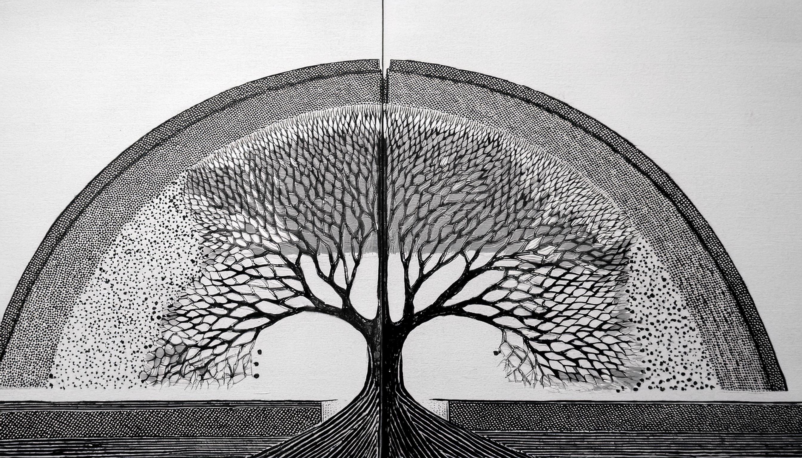
Fibonacci Sequence and the Golden Ratio: Nature’s Architecture
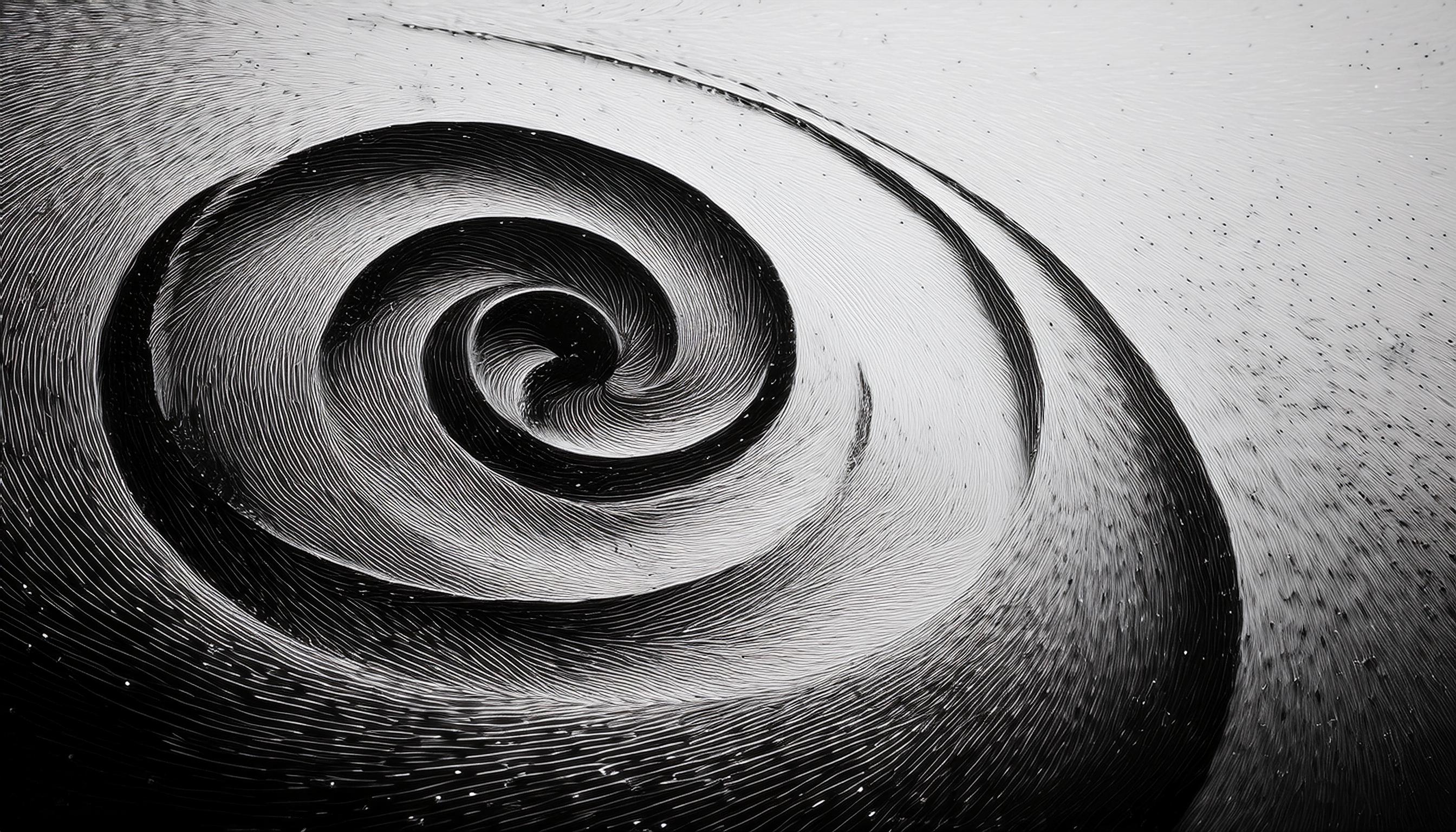
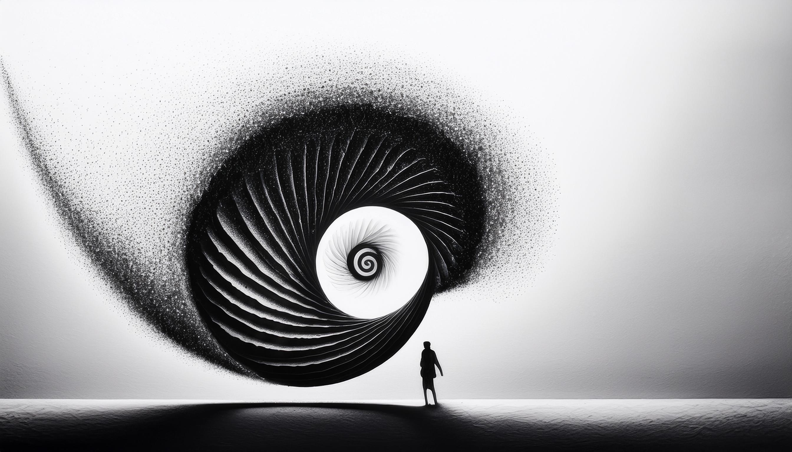
The Fibonacci sequence is one of nature’s most elegant and ubiquitous patterns. This simple sequence, where each number is the sum of the two preceding ones—0, 1, 1, 2, 3, 5, 8, 13, and so on—has a unique property. As it progresses, the ratio between consecutive Fibonacci numbers approaches the Golden Ratio, approximately 1.618. This ratio has fascinated mathematicians, artists, and scientists for centuries, appearing throughout nature and often being associated with visual harmony and beauty.
But what makes this ratio so special? It governs patterns seen everywhere in the natural world. From the spiral of seashells and the arrangement of sunflower seeds to the proportions of the human body, the Golden Ratio appears as if it’s a hidden code, a structural blueprint of beauty that transcends cultural boundaries. Artists and architects have long recognized its aesthetic appeal, using it to create works that feel balanced and pleasing to the eye.
Here, I want to recreate this pattern, not just to explain it but to bring it to life through generative code. By using p5.js, we can construct a visual representation of the Fibonacci spiral, showing how the Golden Ratio emerges naturally and elegantly from simple mathematical rules.
Creating the Fibonacci Spiral with p5.js
Using a few lines of code, we can generate a spiral that follows the Fibonacci sequence, building an ever-expanding pattern that mimics natural forms. In p5.js, this spiral can be created by calculating points along a curve, each point growing based on the sequence.
function setup() {
  createCanvas(400, 400);
  background(255);
  let angle = 0;
  let radius = 5;

  for (let i = 0; i < 20; i++) {
    let x = width / 2 + cos(angle) * radius;
    let y = height / 2 + sin(angle) * radius;

    fill(0);
    ellipse(x, y, radius, radius);

    angle += PI / 5;
    radius += 5;
  }
}
Here’s what the code does: starting from the center of the canvas, each point is positioned along a curve based on an angle and radius that increase with each step. The result is a spiral, a natural and familiar form that grows from a single point into something complex and beautiful. This spiral mimics the structure seen in galaxies, shells, and flowers—an echo of nature’s own architecture.
Experimenting with Parameters
One of the exciting things about using code to generate art is the ability to play with parameters. For instance, changing the angle increment from PI / 5 to PI / 6 adjusts the spacing between points, creating a tighter or looser spiral. Such small modifications can lead to entirely new forms, each one unique but still grounded in the same underlying mathematical principles.
The beauty of the Fibonacci sequence and the Golden Ratio isn’t just in the numbers; it’s in the way these patterns emerge in the natural world, guiding growth and structure in ways that feel instinctively pleasing. Perhaps there’s something in our brains that recognizes this proportion as “right,” as balanced. It’s as if the Golden Ratio is a secret code embedded within us, resonating with our sense of harmony.
Fractals and Self-Similarity: Complexity from Simple Rules
Where the Fibonacci sequence gives us smooth, harmonious curves, fractals take us into the realm of infinitely complex structures. A fractal is a pattern that repeats itself on different scales, each part resembling the whole. This phenomenon, known as self-similarity, is everywhere in nature: it shapes the jagged coastlines of continents, the veins of leaves, the branching of trees, and even the formation of clouds.
Fractals are created through recursion—a process where a pattern is generated by repeating a rule on an increasingly smaller scale. This can result in mind-boggling complexity from the simplest of instructions. Perhaps the most famous example is the Mandelbrot set, a mathematical object that reveals endless detail the closer you look.
Generating a Fractal with p5.js
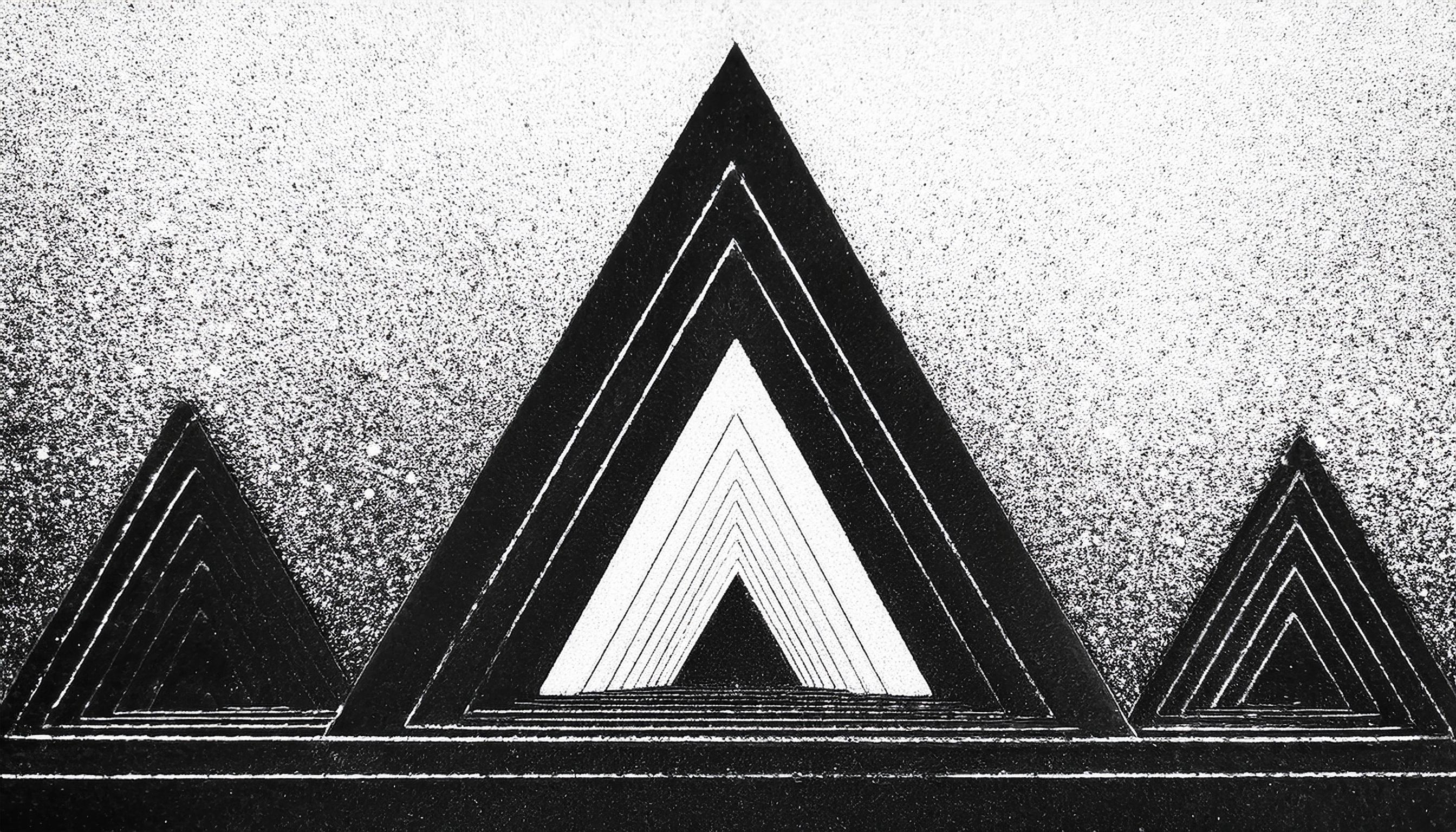
In the digital world, we can create fractals by applying recursive rules through code. Here’s an example in p5.js that uses recursion to generate a basic fractal pattern—the Sierpinski triangle. This fractal is built by dividing a triangle into smaller triangles, over and over, creating a visual that’s both orderly and complex.
function setup() {
  createCanvas(400, 400);
  background(255);
  noFill();
  stroke(0);
  sierpinski(200, 50, 300);
}

function sierpinski(x, y, size) {
  if (size > 10) {
    triangle(x, y, x - size / 2, y + size, x + size / 2, y + size);
    sierpinski(x, y, size / 2);
    sierpinski(x - size / 2, y + size / 2, size / 2);
    sierpinski(x + size / 2, y + size / 2, size / 2);
  }
}
In this code, the sierpinski function is called recursively. Each time it’s called, it divides the current triangle into three smaller ones, adding complexity with each iteration. This simple recursive rule creates a pattern that seems almost organic, like the branching structure of a tree or the layered texture of a mountain range.
Visual Transformation: Before and After
Starting with a single large triangle, the pattern becomes more intricate as the function is applied recursively, transforming the shape into an interconnected network of smaller triangles. The “before” image is just a blank canvas, but as each layer of recursion is added, the triangle fills with detail, demonstrating the natural elegance of self-similarity.
Fractals in Nature
What’s astonishing is that nature follows these same rules. In the structure of rivers, tree branches, and even blood vessels, self-similar patterns emerge. Fractals allow nature to create complexity without needing infinite resources; it’s a simple way of building large structures with small, repeating units. In essence, fractals give life to the saying that “nature is both infinitely complex and infinitely simple.”
Experimenting with Scale and Depth
The depth of recursion determines the detail of the fractal. By increasing or decreasing the recursion depth in the code, we can create a pattern that’s either highly detailed or minimalistic. Adjusting the size parameter also affects the scale, allowing us to control how “zoomed in” the fractal appears.
In the digital realm, fractals offer a visual metaphor for the complexity of the universe—a complexity that arises from surprisingly simple foundations. They remind us that, at the heart of apparent chaos, there is an underlying order, a repetitive structure that mirrors itself across scales.
Fractals are more than just mathematical curiosities; they’re proof that beauty can arise from simplicity. As we create these digital patterns, we’re not just drawing shapes—we’re tapping into the same rules that nature uses to build itself.
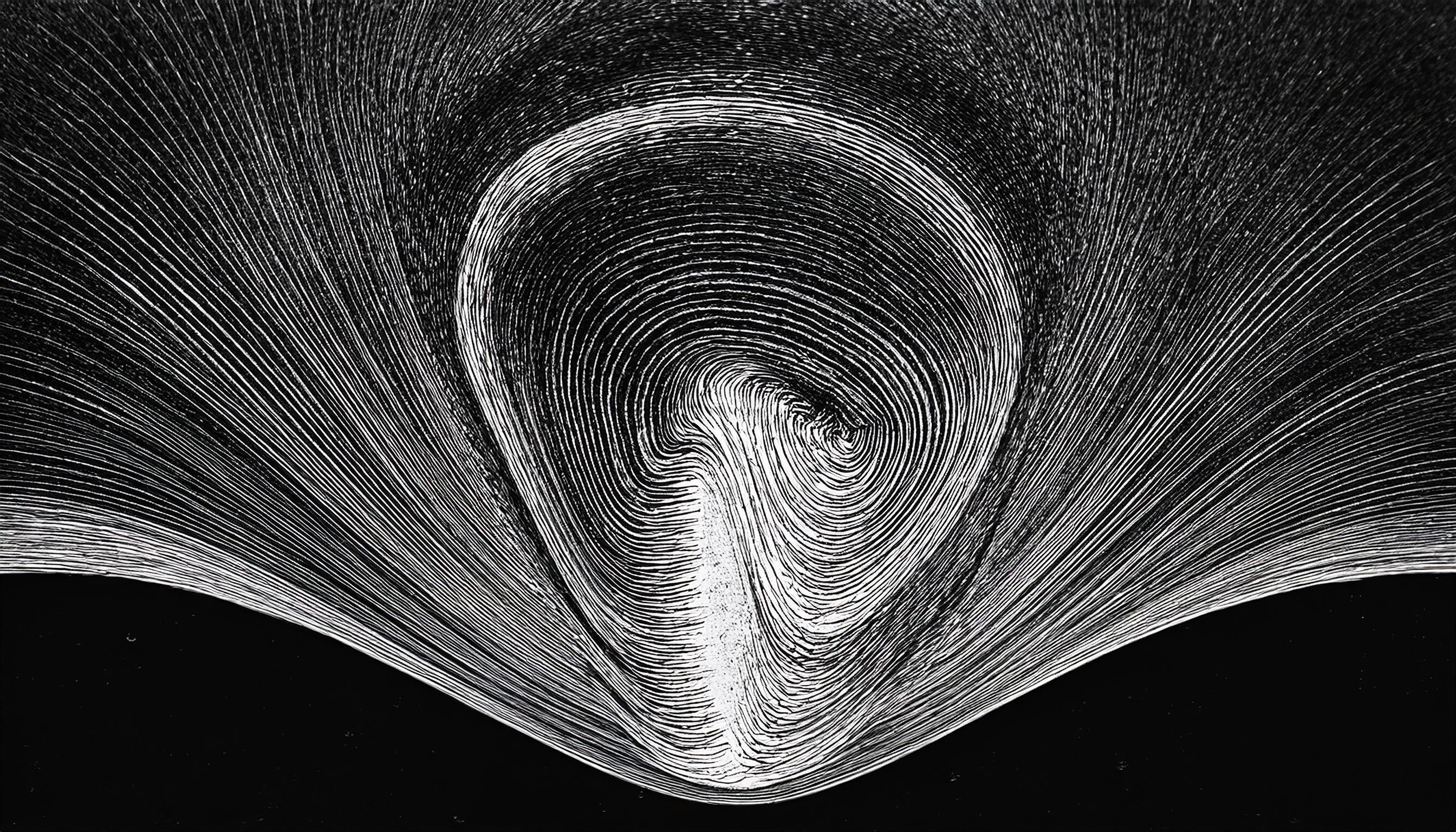
Perlin Noise: Adding Organic Texture to Images
While fractals reveal the complexity of repetition, Perlin noise introduces a different kind of organic structure. Developed by Ken Perlin, this mathematical function creates smooth, random variations that feel natural. Unlike pure randomness, which can appear chaotic and disjointed, Perlin noise transitions gradually from one value to the next, resulting in patterns that mimic natural textures like clouds, waves, or flowing landscapes.
In generative art and computer graphics, Perlin noise is widely used to bring a sense of realism and natural flow to digital creations. Its controlled randomness allows for textures that feel familiar—like the rolling of hills or the drifting of fog. With code, we can apply Perlin noise to an image to transform its appearance, adding a layer of organic texture that gives it a more dynamic, lifelike quality.
Applying Perlin Noise to an Image in p5.js
Rather than starting from scratch, we can take an existing image and overlay it with Perlin noise, altering each pixel in a way that produces a subtle, textured effect. Here’s an example in p5.js that loads an image and then uses Perlin noise to modify its pixels.
let img;

function preload() {
  // Load an image from the editor's directory or a URL
  img = loadImage('path/to/your/image.jpg'); // Replace with the path to your image
}

function setup() {
  createCanvas(400, 400);
  background(255);
  img.resize(width, height); // Resize the image to fit the canvas
  applyPerlinNoise();
}

function applyPerlinNoise() {
  img.loadPixels();

  for (let y = 0; y < img.height; y++) {
    for (let x = 0; x < img.width; x++) {
      // Get the current pixel's color
      let index = (x + y * img.width) * 4;
      let r = img.pixels[index];
      let g = img.pixels[index + 1];
      let b = img.pixels[index + 2];

      // Apply Perlin noise to the color channels
      let noiseVal = noise(x * 0.05, y * 0.05);
      img.pixels[index] = r * noiseVal;
      img.pixels[index + 1] = g * noiseVal;
      img.pixels[index + 2] = b * noiseVal;
    }
  }

  img.updatePixels();
  image(img, 0, 0); // Display the modified image on the canvas
}
In this code, we start by loading an image, resizing it to fit the canvas, and then applying Perlin noise to its pixels. The applyPerlinNoise function processes each pixel, using Perlin noise to adjust its RGB values. This approach adds a textured overlay to the image, giving it a unique, organic quality.
Visual Transformation: Before and After
The effect of Perlin noise on an image is subtle yet powerful. When we start with a plain image, it feels static and defined. But after applying Perlin noise, the image takes on a more dynamic appearance, with each pixel subtly influenced by the noise. The result is a textured look, as though the image has been painted with waves of color, giving it depth and movement.
Experimenting with Scale and Frequency
The parameters within the noise function control the scale and density of the effect. By adjusting values like x * 0.05 and y * 0.05, we can increase or decrease the smoothness of the noise. A lower frequency (e.g., x * 0.01) will produce larger, gentler waves, while a higher frequency (e.g., x * 0.1) creates finer, more intricate patterns.
This flexibility makes Perlin noise a versatile tool in generative art. It allows us to experiment with texture, adding complexity without overwhelming the original form of the image. By applying it to different kinds of visuals, we can create a range of effects—from subtle, grainy textures to bold, wave-like distortions.
The Organic Essence of Controlled Randomness
Perlin noise is more than just a mathematical function; it’s a bridge between the digital and the natural. In the world of computer graphics, it brings a hint of realism to artificial creations, echoing the random-yet-coherent textures we see in nature. This effect reminds us that even chaos can have a certain order, a rhythm that feels familiar to us on a fundamental level.
In this way, applying Perlin noise to an image is not just a transformation—it’s an invitation to see the hidden patterns within randomness, a reminder that even in digital art, we can capture the essence of nature.
Fourier Transform: Decomposing and Reconstructing Patterns
The Fourier Transform is a powerful mathematical tool that allows us to decompose complex signals—like images or sounds—into simpler, sine and cosine components. This decomposition reveals the “frequency” of each component, which can be thought of as the underlying structure or rhythm of the data. In essence, the Fourier Transform lets us look beneath the surface of an image to see its hidden patterns.
In digital art and image processing, the Fourier Transform is often used to analyze textures, apply filters, or even create visually striking distortions. By breaking an image down into frequency components, we can manipulate its structure in ways that are impossible with basic pixel-based transformations.
Step 1: Basic Fourier Analysis
To get started, let’s begin with a simple Fourier analysis of an image using p5.js. We’ll take a straightforward approach, extracting basic frequency information from the image, and display the effect this has visually.
Note: Since p5.js doesn’t natively support Fourier Transforms for images, we’ll start with a simple simulation by adjusting brightness values based on a sine wave, giving us a taste of how frequency manipulation can alter an image.
let img;

function preload() {
  img = loadImage('path/to/your/image.jpg'); // Replace with your image path
}

function setup() {
  createCanvas(400, 400);
  background(255);
  img.resize(width, height);
  applyBasicFourierEffect();
}

function applyBasicFourierEffect() {
  img.loadPixels();

  for (let y = 0; y < img.height; y++) {
    for (let x = 0; x < img.width; x++) {
      let index = (x + y * img.width) * 4;
      let r = img.pixels[index];
      let g = img.pixels[index + 1];
      let b = img.pixels[index + 2];

      // Apply a sine wave to the brightness based on x position
      let brightnessAdjustment = sin(x * 0.1) * 50;
      img.pixels[index] = constrain(r + brightnessAdjustment, 0, 255);
      img.pixels[index + 1] = constrain(g + brightnessAdjustment, 0, 255);
      img.pixels[index + 2] = constrain(b + brightnessAdjustment, 0, 255);
    }
  }

  img.updatePixels();
  image(img, 0, 0);
}
Explanation of the Code
1. Sine Wave Manipulation: In this introductory step, instead of applying a full Fourier Transform, we modify each pixel’s brightness using a sine wave. This simulates the concept of adding a “frequency” to the image, as the sine wave affects brightness values periodically across the x-axis.
2. Constraining Brightness: The constrain function ensures the brightness doesn’t exceed the typical 0–255 range, preventing unintended color distortions.
Visual Transformation: Before and After
The initial image remains visually recognizable, but you’ll notice wave-like “bands” of brightness moving horizontally across it. This effect is subtle but demonstrates how frequencies can influence the texture and appearance of an image.
function applyFourierEffectWithMultipleFrequencies() {
  img.loadPixels();

  for (let y = 0; y < img.height; y++) {
    for (let x = 0; x < img.width; x++) {
      let index = (x + y * img.width) * 4;
      let r = img.pixels[index];
      let g = img.pixels[index + 1];
      let b = img.pixels[index + 2];

      // Combine two sine waves with different frequencies
      let brightnessAdjustment = sin(x * 0.1) * 50 + cos(y * 0.05) * 30;
      img.pixels[index] = constrain(r + brightnessAdjustment, 0, 255);
      img.pixels[index + 1] = constrain(g + brightnessAdjustment, 0, 255);
      img.pixels[index + 2] = constrain(b + brightnessAdjustment, 0, 255);
    }
  }

  img.updatePixels();
  image(img, 0, 0);
}
Explanation of the Code
1. Combining Sine and Cosine Waves: By adding both a sine wave and a cosine wave, each with different frequencies, we create a more intricate brightness adjustment pattern across both the x and y axes. This gives a hint of the complexity of Fourier analysis by layering multiple “frequencies” onto the image.
2. Control Over Frequency and Amplitude: Adjusting the multipliers in sin(x * 0.1) * 50 and cos(y * 0.05) * 30 allows us to control the frequency and amplitude of each wave, adding more flexibility in how the image is altered.
Visual Transformation: Before and After
With two frequencies applied, the effect becomes more pronounced. The image now has a subtle, grid-like overlay where different areas are brightened or darkened based on their position. This effect begins to mimic the idea of decomposing and reconstructing an image with multiple frequency layers.
Step 3: Preparing for a Full Fourier Transform
At this point, we’ve explored how sine and cosine waves can manipulate an image’s brightness to simulate frequency adjustments. To perform a full Fourier Transform on images, we would typically rely on a library capable of handling complex mathematical operations, like the Fast Fourier Transform (FFT). In p5.js, this would require custom code or additional libraries.
However, by experimenting with layered sine and cosine waves, we’ve taken the first steps toward understanding how Fourier analysis reveals the hidden “frequencies” in an image, transforming its structure in visually intriguing ways.
Cellular Automata: Patterns Emerging from Simple Rules
A cellular automaton is a grid of cells that evolve over time based on a set of rules. The cells can be in different states (e.g., on or off, black or white), and each cell’s future state is determined by the states of its neighboring cells. This process creates complex, often self-similar patterns that resemble structures found in nature, like branching trees or the fractal shapes of river networks.
One of the simplest examples of cellular automata is Rule 30, where each cell’s state in the next generation depends on its current state and the states of its immediate neighbors. Despite its simplicity, Rule 30 produces a chaotic, visually complex pattern that spreads across the grid.
Step 1: Implementing Rule 30 in p5.js
In our first step, let’s implement Rule 30 in a 1-dimensional cellular automaton, where each row represents the next generation based on the rules applied to the previous row.
let cells = [];
let cellSize = 10;
let generation = 0;

function setup() {
  createCanvas(400, 400);
  background(255);

  // Initialize the cells array with all cells "off" except the center cell
  cells = Array(floor(width / cellSize)).fill(0);
  cells[floor(cells.length / 2)] = 1; // Center cell is "on"
}

function draw() {
  // Draw the current generation of cells
  for (let i = 0; i < cells.length; i++) {
    if (cells[i] == 1) fill(0); // Black for "on" cells
    else fill(255); // White for "off" cells
    rect(i * cellSize, generation * cellSize, cellSize, cellSize);
  }

  // Generate the next generation
  let nextGen = Array(cells.length).fill(0);
  for (let i = 1; i < cells.length - 1; i++) {
    let left = cells[i - 1];
    let center = cells[i];
    let right = cells[i + 1];

    // Apply Rule 30
    if ((left == 1 && center == 0 && right == 0) ||
        (left == 0 && center == 1 && right == 1) ||
        (left == 0 && center == 1 && right == 0) ||
        (left == 0 && center == 0 && right == 1)) {
      nextGen[i] = 1;
    }
  }

  // Update cells to the next generation and move to the next row
  cells = nextGen;
  generation++;

  // Stop when we reach the bottom of the canvas
  if (generation * cellSize >= height) noLoop();
}
Explanation of the Code
1. Initialization: We create an array cells that represents the states of each cell in a row. All cells are initially “off” (0), except for the center cell, which is “on” (1).
2. Rule 30 Logic: For each cell, we check the state of its left, center, and right neighbors to determine its next state. This rule creates a chaotic, branching pattern as the generations progress.
3. Drawing the Grid: Each cell is displayed as a black or white rectangle, with each new generation of cells being drawn in the next row.
Visual Transformation: Before and After
Starting with a single cell turned on in the center, Rule 30 quickly creates a complex triangular pattern as it iterates through each generation. What begins as a simple line soon becomes a structured but chaotic tapestry of black and white cells.
Step 2: Increasing Complexity with Multiple Rules
Now, let’s increase the complexity slightly by implementing a different rule, Rule 90, alongside Rule 30. We’ll add an option to switch between the two rules, demonstrating how small changes in the rule set can drastically alter the pattern.
let rule = 30; // You can change this to 90 for Rule 90

function applyRule(left, center, right) {
  if (rule == 30) {
    // Rule 30 logic
    return (left == 1 && center == 0 && right == 0) ||
           (left == 0 && center == 1 && right == 1) ||
           (left == 0 && center == 1 && right == 0) ||
           (left == 0 && center == 0 && right == 1) ? 1 : 0;
  } else if (rule == 90) {
    // Rule 90 logic
    return left ^ right; // XOR operation for Rule 90
  }
}

function draw() {
  for (let i = 0; i < cells.length; i++) {
    fill(cells[i] == 1 ? 0 : 255);
    rect(i * cellSize, generation * cellSize, cellSize, cellSize);
  }

  let nextGen = Array(cells.length).fill(0);
  for (let i = 1; i < cells.length - 1; i++) {
    let left = cells[i - 1];
    let center = cells[i];
    let right = cells[i + 1];

    nextGen[i] = applyRule(left, center, right);
  }

  cells = nextGen;
  generation++;

  if (generation * cellSize >= height) noLoop();
}
Explanation of the Code Changes
1. Rule Selection: We introduce a variable rule that allows us to switch between Rule 30 and Rule 90.
2. Rule Logic Function: The applyRule function now contains the logic for both Rule 30 and Rule 90, selected based on the rule variable.
3. Rule 90 Behavior: Rule 90 uses an XOR (exclusive OR) operation between the left and right neighbors, which creates a pattern resembling Sierpinski triangles, distinct from the chaotic structure of Rule 30.
Visual Transformation: Different Patterns from Different Rules
The ability to switch between Rule 30 and Rule 90 demonstrates how a simple change in rules leads to dramatically different visual outcomes. While Rule 30 produces a chaotic, natural-looking pattern, Rule 90 creates a highly structured, fractal-like design. This versatility shows how cellular automata can serve as a tool for generating a wide range of complex patterns from minimal instructions.
Step 3: Expanding to 2D Cellular Automata
Finally, let’s move from a 1D cellular automaton to a 2D version. In 2D cellular automata, each cell is influenced by the eight surrounding cells, rather than just neighbors on either side. This creates an even richer pattern that can resemble things like coral growth, fire, or even cellular life forms.

Now we’ll explore 2D Cellular Automata. In this version, each cell’s state will depend on its eight neighbors, resulting in far more complex and visually engaging patterns than in the 1D version.
For this example, we’ll implement a basic form of Conway’s Game of Life, one of the most well-known 2D cellular automata. In Conway’s Game of Life, each cell follows these simple rules:
1. Underpopulation: If a cell is “on” and has fewer than two “on” neighbors, it turns “off” in the next generation.
2. Survival: If a cell is “on” and has two or three “on” neighbors, it stays “on.”
3. Overpopulation: If a cell is “on” and has more than three “on” neighbors, it turns “off.”
4. Reproduction: If a cell is “off” and has exactly three “on” neighbors, it turns “on.”
These rules create dynamic, evolving patterns that look almost lifelike as clusters grow, merge, and disappear over time.
Step 1: Basic Setup for Conway’s Game of Life
Let’s start with a foundational version of Conway’s Game of Life in p5.js, where each cell’s state will depend on the states of its eight neighboring cells.
let grid;
let cols, rows;
let cellSize = 10;

function setup() {
  createCanvas(400, 400);
  cols = width / cellSize;
  rows = height / cellSize;

  // Initialize grid with random states (on or off)
  grid = Array.from({ length: cols }, () => Array(rows).fill(0).map(() => floor(random(2))));
  frameRate(10); // Slow down to observe evolution
}

function draw() {
  background(255);

  // Display the grid
  for (let x = 0; x < cols; x++) {
    for (let y = 0; y < rows; y++) {
      fill(grid[x][y] === 1 ? 0 : 255);
      stroke(200);
      rect(x * cellSize, y * cellSize, cellSize, cellSize);
    }
  }

  // Calculate the next generation
  let nextGrid = Array.from({ length: cols }, () => Array(rows).fill(0));

  for (let x = 0; x < cols; x++) {
    for (let y = 0; y < rows; y++) {
      let neighbors = countNeighbors(grid, x, y);

      // Apply Conway's Game of Life rules
      if (grid[x][y] === 1) {
        nextGrid[x][y] = (neighbors === 2 || neighbors === 3) ? 1 : 0;
      } else {
        nextGrid[x][y] = (neighbors === 3) ? 1 : 0;
      }
    }
  }

  // Update grid
  grid = nextGrid;
}

// Count "on" neighbors for a given cell
function countNeighbors(grid, x, y) {
  let sum = 0;
  for (let i = -1; i <= 1; i++) {
    for (let j = -1; j <= 1; j++) {
      let col = (x + i + cols) % cols;
      let row = (y + j + rows) % rows;
      sum += grid[col][row];
    }
  }
  sum -= grid[x][y]; // Subtract the cell itself
  return sum;
}
Explanation of the Code
1. Grid Initialization: We create a 2D array grid where each cell is initialized randomly to either “on” (1) or “off” (0).
2. Display: Each cell is drawn as a black or white square, depending on its state.
3. Neighbor Counting: The countNeighbors function calculates the number of “on” neighbors for each cell, taking into account wrap-around edges to create a toroidal (donut-like) grid.
4. Conway’s Rules: For each cell, we apply the Game of Life rules based on the count of neighboring cells. Cells either stay “on,” turn “off,” or switch “on” depending on the number of active neighbors.
5. Updating the Grid: After calculating the next generation, the grid is updated, creating a continuously evolving pattern.
Visual Transformation: Before and After
With this setup, random initial patterns evolve over time, creating clusters that grow, move, and disappear according to Conway’s rules. The resulting patterns resemble life-like structures—some formations stabilize, others oscillate or travel across the grid, while some simply fade out.
Step 2: Adding Interactivity and Complexity
To make the cellular automaton more engaging, let’s add some interactivity. For instance, we could allow the user to click to toggle cells “on” or “off,” enabling them to create initial patterns manually. Additionally, we’ll add a “clear” and “reset” button to start new patterns.
let grid;
let cols, rows;
let cellSize = 10;

function setup() {
  createCanvas(400, 400);
  cols = width / cellSize;
  rows = height / cellSize;
  grid = Array.from({ length: cols }, () => Array(rows).fill(0));
  createButton('Clear').mousePressed(clearGrid);
  createButton('Randomize').mousePressed(randomizeGrid);
  frameRate(10);
}

function draw() {
  background(255);
  for (let x = 0; x < cols; x++) {
    for (let y = 0; y < rows; y++) {
      fill(grid[x][y] === 1 ? 0 : 255);
      stroke(200);
      rect(x * cellSize, y * cellSize, cellSize, cellSize);
    }
  }
  if (mouseIsPressed) {
    let x = floor(mouseX / cellSize);
    let y = floor(mouseY / cellSize);
    if (x >= 0 && x < cols && y >= 0 && y < rows) {
      grid[x][y] = grid[x][y] === 1 ? 0 : 1; // Toggle cell state
    }
  }
  let nextGrid = Array.from({ length: cols }, () => Array(rows).fill(0));
  for (let x = 0; x < cols; x++) {
    for (let y = 0; y < rows; y++) {
      let neighbors = countNeighbors(grid, x, y);
      if (grid[x][y] === 1) {
        nextGrid[x][y] = (neighbors === 2 || neighbors === 3) ? 1 : 0;
      } else {
        nextGrid[x][y] = (neighbors === 3) ? 1 : 0;
      }
    }
  }
  grid = nextGrid;
}

function clearGrid() {
  grid = Array.from({ length: cols }, () => Array(rows).fill(0));
}

function randomizeGrid() {
  grid = Array.from({ length: cols }, () => Array(rows).fill(0).map(() => floor(random(2))));
}
Explanation of the Enhancements
1. Interactive Cell Toggling: Users can now click on cells to toggle them “on” or “off,” allowing for manual pattern creation.
2. Clear and Randomize Buttons: The “Clear” button resets all cells to “off,” while “Randomize” generates a new random pattern, providing more control over the initial conditions.
Results
This interactive version allows for experimentation with different patterns. Users can create custom initial states, watch them evolve, and reset as desired, making the process more engaging and exploratory.

Voronoi Diagrams: Dividing Space in Natural Patterns
A Voronoi diagram partitions a plane into regions based on proximity to a set of points. Each point has a “cell” around it, consisting of all the points in space that are closer to it than to any other point. This kind of partitioning occurs naturally and often produces visually pleasing, organic shapes.
Voronoi diagrams are widely used in fields like computational geometry, biology, and architecture, where dividing space efficiently and organically is important. In generative art, Voronoi cells can create captivating, almost mosaic-like compositions.
Step 1: Basic Static Voronoi Diagram with Random Points
To begin, let’s create a static Voronoi diagram by generating a set of random points on the canvas and coloring each region based on the nearest point.
let points = [];
let numPoints = 10;

function setup() {
  createCanvas(400, 400);
  for (let i = 0; i < numPoints; i++) {
    points.push(createVector(random(width), random(height)));
  }
  noLoop();
}

function draw() {
  for (let x = 0; x < width; x++) {
    for (let y = 0; y < height; y++) {
      let closestPoint = -1;
      let closestDist = Infinity;

      // Find the nearest point
      for (let i = 0; i < points.length; i++) {
        let d = dist(x, y, points[i].x, points[i].y);
        if (d < closestDist) {
          closestDist = d;
          closestPoint = i;
        }
      }

      // Color each pixel based on the closest point
      stroke((closestPoint * 50) % 255, (closestPoint * 100) % 255, 200);
      point(x, y);
    }
  }

  // Draw points on top
  fill(0);
  for (let p of points) {
    ellipse(p.x, p.y, 5, 5);
  }
}
Explanation of the Code
1. Random Points Generation: We generate a set of random points that will act as the centers for our Voronoi cells.
2. Distance Calculation: For each pixel, we calculate the distance to each point and find the closest point. This determines the cell each pixel belongs to.
3. Coloring Cells: Each pixel is colored based on the index of the nearest point, creating a patchwork of regions around each point. By assigning colors based on the closest point, we form the distinct Voronoi cells.
Visual Transformation: Static Voronoi Diagram
The static Voronoi diagram resembles a mosaic, with each cell shaped according to the position of the points. Each cell expands outward until it meets the boundary of a neighboring cell, creating a balanced yet irregular pattern.
Step 2: Dynamic Voronoi Diagram with Moving Points
Now, let’s add some dynamism by making the points move randomly over time. This will cause the cells to shift and morph, creating a constantly evolving Voronoi diagram.
function setup() {
  createCanvas(400, 400);
  for (let i = 0; i < numPoints; i++) {
    points.push(createVector(random(width), random(height)));
  }
}

function draw() {
  background(255);

  // Calculate Voronoi cells
  for (let x = 0; x < width; x++) {
    for (let y = 0; y < height; y++) {
      let closestPoint = -1;
      let closestDist = Infinity;
      for (let i = 0; i < points.length; i++) {
        let d = dist(x, y, points[i].x, points[i].y);
        if (d < closestDist) {
          closestDist = d;
          closestPoint = i;
        }
      }
      stroke((closestPoint * 50) % 255, (closestPoint * 100) % 255, 200);
      point(x, y);
    }
  }

  // Draw and move points
  fill(0);
  for (let p of points) {
    ellipse(p.x, p.y, 5, 5);
    p.x += random(-1, 1);
    p.y += random(-1, 1);
  }
}
Explanation of the Code Adjustments
1. Moving Points: In each frame, the points move slightly in random directions, causing the Voronoi cells to shift and morph.
2. Dynamic Rendering: We call draw() repeatedly, allowing the cells to change dynamically as the points move.
Visual Transformation: Dynamic Voronoi Diagram
With moving points, the Voronoi diagram becomes a living, breathing pattern. The cells fluctuate and morph, resembling a shifting mosaic or an abstract, organic structure. This effect gives the sense of something alive, a dynamic partitioning of space that responds to the motion of its points.
Step 3: Adding Color Gradients for Depth
To make the visualization even more visually compelling, we can add color gradients within each cell. By calculating a gradient based on the distance to the nearest point, we create a sense of depth and shading within each Voronoi cell.
function draw() {
  background(255);

  // Calculate Voronoi cells with gradients
  for (let x = 0; x < width; x++) {
    for (let y = 0; y < height; y++) {
      let closestPoint = -1;
      let closestDist = Infinity;
      for (let i = 0; i < points.length; i++) {
        let d = dist(x, y, points[i].x, points[i].y);
        if (d < closestDist) {
          closestDist = d;
          closestPoint = i;
        }
      }

      // Apply color gradient based on distance to closest point
      let colorIntensity = map(closestDist, 0, 100, 255, 150); // Adjust gradient scale
      stroke((closestPoint * 50) % 255, colorIntensity, 200);
      point(x, y);
    }
  }

  // Draw and move points
  fill(0);
  for (let p of points) {
    ellipse(p.x, p.y, 5, 5);
    p.x += random(-1, 1);
    p.y += random(-1, 1);
  }
}
Explanation of the Gradient Enhancement
1. Distance-Based Color Gradient: We map the closestDist to a color intensity, creating a gradient effect within each Voronoi cell. Cells are darker near the center point and gradually lighten toward the edges.
2. Visual Depth: The gradient effect adds depth, making each cell feel more three-dimensional. This simple addition creates a more sophisticated, polished look.
Result: A Dynamic, Gradient-Enhanced Voronoi Diagram
The final product is a dynamic Voronoi diagram with color gradients that give each cell a sense of depth. The cells shift and flow as the points move, creating an intricate and ever-evolving partitioning of space. This kind of pattern resembles biological textures or abstract, organic forms, illustrating the beauty of Voronoi structures in a visually engaging way.
Let’s explore Chaos Theory and the concept of Order Within Chaos. Chaos theory is the study of systems that are highly sensitive to initial conditions, where small changes can lead to vastly different outcomes. This phenomenon is often referred to as the “butterfly effect,” where even the smallest disturbance can cascade into larger, unpredictable changes.
In generative art and mathematical simulations, chaos theory helps us understand how seemingly random patterns can have underlying structures and order. In this section, we’ll use p5.js to create a chaotic system that produces beautiful, intricate patterns—specifically, a double pendulum. This is a classic example of a chaotic system, where the movement of one pendulum affects the other, creating a path that is both unpredictable and captivating.
We’ll start with a basic double pendulum and progressively add complexity, allowing for a more visually engaging, chaotic pattern.
Chaos Theory: The Beauty of a Double Pendulum
A double pendulum consists of one pendulum attached to the end of another. The motion of the double pendulum is governed by physics but is extremely sensitive to initial conditions. Even a slight change in the starting angle or velocity can produce a drastically different motion, making it an excellent example of chaos in action.
Step 1: Basic Double Pendulum Simulation
To begin, we’ll create a simple double pendulum in p5.js. We’ll start by defining the lengths and masses of the two pendulums and then calculate their positions based on basic physics equations.
let r1 = 125; // Length of the first rod
let r2 = 125; // Length of the second rod
let m1 = 10;  // Mass of the first pendulum
let m2 = 10;  // Mass of the second pendulum
let a1 = Math.PI / 2; // Angle of the first pendulum
let a2 = Math.PI / 2; // Angle of the second pendulum
let a1_v = 0; // Angular velocity of the first pendulum
let a2_v = 0; // Angular velocity of the second pendulum
let g = 1;    // Gravity

let px2 = -1;
let py2 = -1;

function setup() {
  createCanvas(400, 400);
  background(255);
}

function draw() {
  // Calculate positions of the two pendulums
  let num1 = -g * (2 * m1 + m2) * sin(a1);
  let num2 = -m2 * g * sin(a1 - 2 * a2);
  let num3 = -2 * sin(a1 - a2) * m2;
  let num4 = a2_v * a2_v * r2 + a1_v * a1_v * r1 * cos(a1 - a2);
  let den = r1 * (2 * m1 + m2 - m2 * cos(2 * a1 - 2 * a2));
  let a1_a = (num1 + num2 + num3 * num4) / den;

  num1 = 2 * sin(a1 - a2);
  num2 = (a1_v * a1_v * r1 * (m1 + m2));
  num3 = g * (m1 + m2) * cos(a1);
  num4 = a2_v * a2_v * r2 * m2 * cos(a1 - a2);
  den = r2 * (2 * m1 + m2 - m2 * cos(2 * a1 - 2 * a2));
  let a2_a = (num1 * (num2 + num3 + num4)) / den;

  // Update velocities and angles
  a1_v += a1_a;
  a2_v += a2_a;
  a1 += a1_v;
  a2 += a2_v;

  // Damping to slow down the motion
  a1_v *= 0.99;
  a2_v *= 0.99;

  // Calculate x and y positions
  let x1 = r1 * sin(a1);
  let y1 = r1 * cos(a1);
  let x2 = x1 + r2 * sin(a2);
  let y2 = y1 + r2 * cos(a2);

  // Draw the path of the second pendulum
  stroke(0, 50);
  if (px2 !== -1 && py2 !== -1) {
    line(px2 + width / 2, py2 + height / 2, x2 + width / 2, y2 + height / 2);
  }

  // Update previous positions
  px2 = x2;
  py2 = y2;

  // Draw the pendulums
  fill(0);
  stroke(0);
  line(width / 2, height / 2, x1 + width / 2, y1 + height / 2);
  ellipse(x1 + width / 2, y1 + height / 2, m1, m1);
  line(x1 + width / 2, y1 + height / 2, x2 + width / 2, y2 + height / 2);
  ellipse(x2 + width / 2, y2 + height / 2, m2, m2);
}
Explanation of the Code
1. Pendulum Properties: We define the lengths, masses, and initial angles for the two pendulums. These properties determine the motion of the system.
2. Calculating Angular Acceleration: The code uses trigonometric calculations based on the equations of motion for a double pendulum. This is where the chaos emerges: small changes in these values produce vastly different results over time.
3. Updating Position: The positions of the pendulums are updated based on their velocities, and a slight damping effect slows the motion gradually.
Visual Transformation: Chaotic Motion of the Double Pendulum
As the pendulum moves, it traces out a path that appears random yet structured, creating looping, overlapping lines. Each run of the code produces a unique pattern due to the chaotic sensitivity of the system. This path is an example of order within chaos, where the pendulum’s motion follows deterministic rules but results in unpredictable behavior.
Step 2: Adding Color to Track Motion Over Time
To highlight the motion path more vividly, let’s add a gradient color trail that changes as the pendulum moves. This will give a sense of time passing, as colors shift along the path.
let hue = 0;

function draw() {
  let num1 = -g * (2 * m1 + m2) * sin(a1);
  let num2 = -m2 * g * sin(a1 - 2 * a2);
  let num3 = -2 * sin(a1 - a2) * m2;
  let num4 = a2_v * a2_v * r2 + a1_v * a1_v * r1 * cos(a1 - a2);
  let den = r1 * (2 * m1 + m2 - m2 * cos(2 * a1 - 2 * a2));
  let a1_a = (num1 + num2 + num3 * num4) / den;

  num1 = 2 * sin(a1 - a2);
  num2 = (a1_v * a1_v * r1 * (m1 + m2));
  num3 = g * (m1 + m2) * cos(a1);
  num4 = a2_v * a2_v * r2 * m2 * cos(a1 - a2);
  den = r2 * (2 * m1 + m2 - m2 * cos(2 * a1 - 2 * a2));
  let a2_a = (num1 * (num2 + num3 + num4)) / den;

  a1_v += a1_a;
  a2_v += a2_a;
  a1 += a1_v;
  a2 += a2_v;

  a1_v *= 0.99;
  a2_v *= 0.99;

  let x1 = r1 * sin(a1);
  let y1 = r1 * cos(a1);
  let x2 = x1 + r2 * sin(a2);
  let y2 = y1 + r2 * cos(a2);

  colorMode(HSB, 255);
  stroke(hue % 255, 255, 255, 50);
  hue += 1;

  if (px2 !== -1 && py2 !== -1) {
    line(px2 + width / 2, py2 + height / 2, x2 + width / 2, y2 + height / 2);
  }

  px2 = x2;
  py2 = y2;

  fill(0);
  stroke(0);
  line(width / 2, height / 2, x1 + width / 2, y1 + height / 2);
  ellipse(x1 + width / 2, y1 + height / 2, m1, m1);
  line(x1 + width / 2, y1 + height / 2, x2 + width / 2, y2 + height / 2);
  ellipse(x2 + width / 2, y2 + height / 2, m2, m2);
}
Explanation of the Color Enhancement
1. Color Gradient: We use the HSB color mode to create a color gradient, cycling through hues as the pendulum moves. This highlights the chaotic path over time and gives a visual representation of the progression of motion.
2. Time-Based Hue Change: By incrementing the hue, each part of the path has a slightly different color, creating a vivid trail that adds depth and energy to the chaotic motion.
Result: An Engaging, Colorful Chaotic Pattern
The final result is a mesmerizing, colorful trail that visualizes the motion of the double pendulum. Each path is unique and unpredictable, providing a beautiful example of chaos theory in action. As the pendulum swings, it reveals both structure and randomness, embodying the complex beauty of chaos.
Now, let’s dive into L-Systems (Lindenmayer Systems), another fascinating tool for creating complex, natural-looking patterns through simple, rule-based instructions. L-systems are widely used in generative art, particularly for simulating the growth patterns of plants and other fractal-like structures.
In an L-system, we start with an initial “axiom” (a simple string of symbols) and apply a set of production rules to expand this string into a more complex one. This string is then interpreted visually, often by using symbols to represent movements (e.g., forward, turn left, turn right), resulting in intricate, recursive shapes.
In this section, we’ll build an L-system from scratch in p5.js, beginning with a basic setup and gradually adding complexity.
L-Systems: Growing Patterns from Simple Rules
L-systems use recursive rules to create complex structures. This method is similar to how plants grow: a seed (or axiom) grows into branches, which in turn grow smaller branches, and so on. Each generation applies rules to the previous one, creating more detailed and complex patterns with each iteration.
Let’s start by implementing a basic L-system that generates a branching pattern.
Step 1: Basic L-System with a Simple Axiom and Rules
To begin, we’ll create a simple L-system that produces a branching pattern based on an initial axiom and a set of production rules. We’ll use the following rules:
• Axiom: F (the initial symbol to start with)
• Rule: F -> F[+F]F[-F]F
• F means “move forward and draw a line”
• + means “turn right”
• – means “turn left”
• [ and ] are used to save and restore the position, allowing for branching
Here’s the basic setup in p5.js:
let axiom = "F";
let sentence = axiom;
let rules = [];
let len = 100;

function setup() {
  createCanvas(400, 400);
  background(255);

  rules[0] = {
    predecessor: "F",
    successor: "F[+F]F[-F]F"
  };

  generate();
  turtle();
}

function generate() {
  let nextSentence = "";
  for (let i = 0; i < sentence.length; i++) {
    let current = sentence.charAt(i);
    let found = false;
    for (let j = 0; j < rules.length; j++) {
      if (current === rules[j].predecessor) {
        nextSentence += rules[j].successor;
        found = true;
        break;
      }
    }
    if (!found) {
      nextSentence += current;
    }
  }
  sentence = nextSentence;
  len *= 0.5; // Shorten the length with each generation for realism
}

function turtle() {
  resetMatrix();
  translate(width / 2, height);
  stroke(0);
  for (let i = 0; i < sentence.length; i++) {
    let current = sentence.charAt(i);

    if (current === "F") {
      line(0, 0, 0, -len);
      translate(0, -len);
    } else if (current === "+") {
      rotate(PI / 6);
    } else if (current === "-") {
      rotate(-PI / 6);
    } else if (current === "[") {
      push();
    } else if (current === "]") {
      pop();
    }
  }
}
Explanation of the Code
1. Axiom and Rules: We define an initial axiom, F, and a rule that replaces F with F[+F]F[-F]F. Each generation applies this rule, creating an increasingly complex string.
2. Generating the Sentence: In generate(), we iterate through each character in sentence, replacing F with the defined rule, thus expanding the sentence over multiple generations.
3. Drawing with Turtle Graphics: The turtle() function interprets the expanded string by moving and rotating based on each symbol, creating a branching pattern. push() and pop() are used to save and restore positions, enabling branching.
Visual Transformation: A Simple Branching Structure
The initial pattern resembles a tree-like structure, with each iteration producing more branches. As the sentence expands, the pattern becomes more intricate, mimicking the way plants branch out as they grow.
Step 2: Adding Multiple Generations
To create more detailed and complex structures, we’ll call generate() multiple times, adding a button to control the number of generations. Each generation will increase the complexity of the pattern.
function setup() {
  createCanvas(400, 400);
  background(255);
  let button = createButton("Generate");
  button.mousePressed(() => {
    generate();
    background(255);
    turtle();
  });

  rules[0] = {
    predecessor: "F",
    successor: "F[+F]F[-F]F"
  };

  turtle();
}
Explanation of the Enhancement
1. Button to Control Generations: We add a button labeled “Generate” to apply the rule and add another generation to the pattern with each click.
2. Complexity Growth: Each time generate() is called, the sentence expands, and the pattern becomes more intricate, creating denser branching with each generation.
Visual Transformation: Increasingly Detailed Branching
With each click, the branching structure becomes more complex, adding layers of detail. The pattern begins to resemble the fractal-like growth of a plant or coral, demonstrating how simple rules can produce intricate forms.
Step 3: Adding Randomness to Mimic Natural Growth
To make the pattern look even more organic, we can introduce slight randomness in the angle of rotation and the length of each branch. This will give the pattern a more natural feel, as real plants rarely grow with perfect symmetry.
function turtle() {
  resetMatrix();
  translate(width / 2, height);
  stroke(0);
  for (let i = 0; i < sentence.length; i++) {
    let current = sentence.charAt(i);

    if (current === "F") {
      line(0, 0, 0, -len * random(0.9, 1.1)); // Randomize branch length
      translate(0, -len * random(0.9, 1.1));
    } else if (current === "+") {
      rotate(PI / 6 * random(0.8, 1.2)); // Randomize angle slightly
    } else if (current === "-") {
      rotate(-PI / 6 * random(0.8, 1.2));
    } else if (current === "[") {
      push();
    } else if (current === "]") {
      pop();
    }
  }
}
Explanation of the Randomization
1. Random Branch Length: By slightly randomizing the length of each F segment, we avoid the uniformity of perfectly identical branches, making the structure look more natural.
2. Random Rotation: A small random factor in the rotation angle (PI / 6 * random(0.8, 1.2)) introduces asymmetry, further enhancing the organic appearance.
Result: An Organic, Tree-Like Structure
With the addition of randomness, the final L-system pattern looks more like a real plant or coral structure. Each branch has slight variations in length and angle, creating an organic, natural appearance. This pattern reveals how order and chaos can coexist, creating visually captivating forms from simple, rule-based systems.
Let’s move into Attractors and specifically explore the Lorenz Attractor, which is a famous example of a chaotic system that exhibits complex, looping behavior. Attractors in general describe the tendency of a system to evolve toward certain patterns or states, even within chaotic dynamics. The Lorenz Attractor is particularly interesting because it creates a “butterfly” shape, which has become a symbol of chaos theory.
In this section, we’ll create a visual representation of the Lorenz Attractor using p5.js. We’ll start with the basic equations to model the attractor, then add visual enhancements as we proceed.
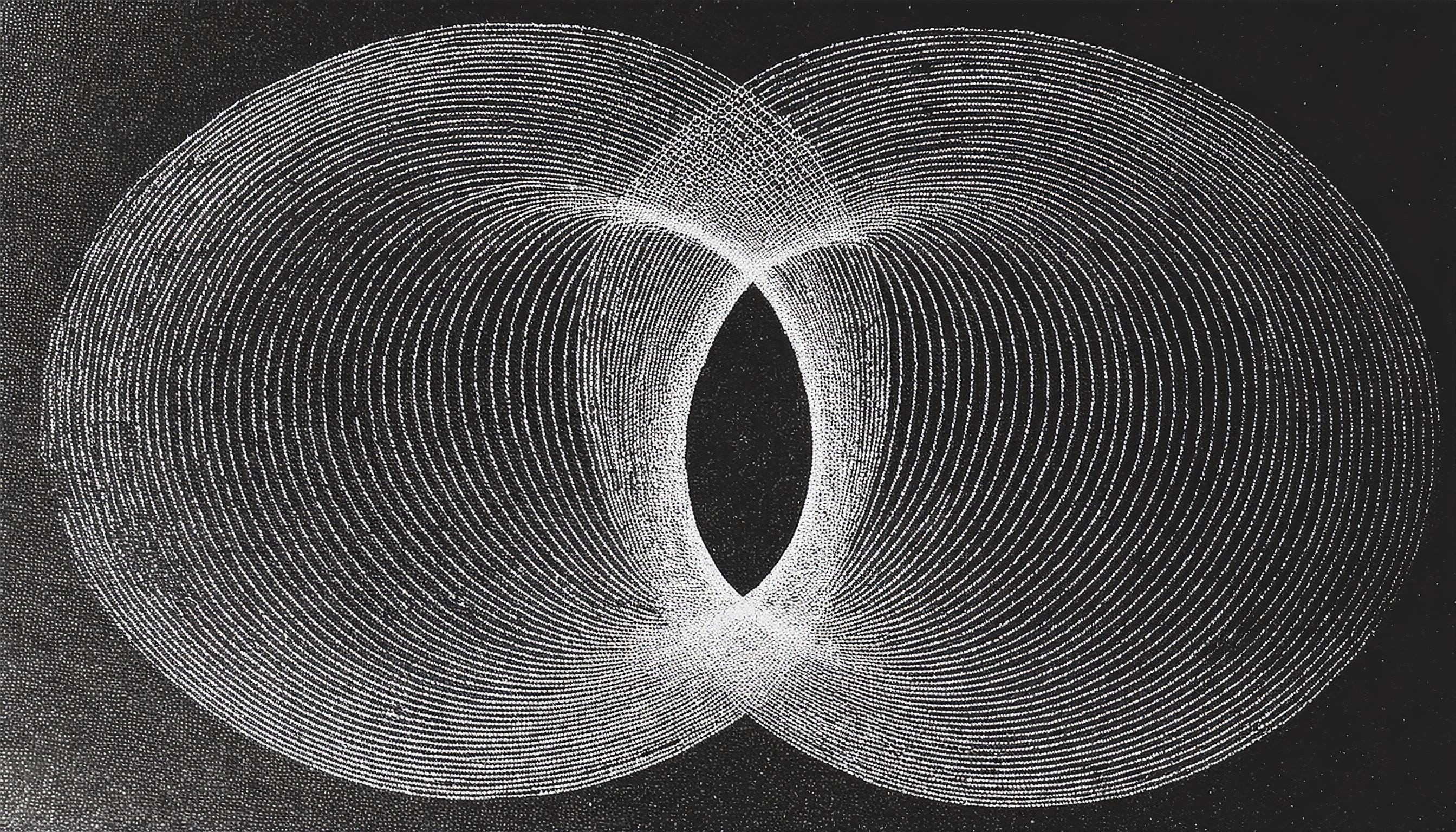
The Lorenz Attractor: Visualizing Chaos in Motion
The Lorenz Attractor was developed by meteorologist Edward Lorenz while studying atmospheric convection. It’s defined by a set of three differential equations that describe the system’s movement in three-dimensional space. These equations are:
1. dx/dt = σ(y – x)
2. dy/dt = x(ρ – z) – y
3. dz/dt = xy – βz
In these equations, σ (sigma), ρ (rho), and β (beta) are constants that influence the attractor’s behavior. For specific values, such as σ = 10, ρ = 28, and β = 8/3, the system produces a chaotic, looping pattern that resembles a butterfly.
Step 1: Implementing the Basic Lorenz Attractor in p5.js
To begin, let’s create a simple simulation of the Lorenz Attractor. We’ll calculate the changes in x, y, and z over time and plot each point to visualize the attractor.
let x = 0.01;
let y = 0;
let z = 0;
let sigma = 10;
let rho = 28;
let beta = 8 / 3;
let points = [];

function setup() {
  createCanvas(600, 600, WEBGL);
  colorMode(HSB);
  background(0);
}

function draw() {
  // Lorenz Attractor equations
  let dt = 0.01;
  let dx = sigma * (y - x) * dt;
  let dy = (x * (rho - z) - y) * dt;
  let dz = (x * y - beta * z) * dt;

  x += dx;
  y += dy;
  z += dz;

  points.push(createVector(x, y, z));

  // Draw the points
  scale(5);
  translate(0, 0, -80);
  stroke(255);
  noFill();
  beginShape();
  for (let v of points) {
    stroke((v.z * 2 + frameCount) % 255, 255, 255); // Color based on z and frame count for a gradient effect
    vertex(v.x, v.y, v.z);
  }
  endShape();
}
Explanation of the Code
1. Initial Conditions and Constants: We initialize x, y, and z with small values, and set up the constants sigma, rho, and beta according to the classic Lorenz Attractor values.
2. Differential Equations: In the draw() function, we calculate the changes in x, y, and z using the Lorenz equations. These values are updated iteratively to trace the path of the attractor.
3. Storing Points: Each new (x, y, z) coordinate is stored in an array points, allowing us to render the full path of the attractor over time.
4. Drawing the Path: We use vertex() to connect each point, creating a continuous, looping path. The color changes gradually based on z and frame count, adding a gradient effect.
Visual Transformation: The Chaotic Butterfly
As the attractor evolves, it creates a mesmerizing, looping structure that traces the chaotic motion of the system. The result is a “butterfly” shape that emerges naturally from the Lorenz equations. This pattern is highly sensitive to initial conditions, meaning even slight changes in the starting values would produce a different trajectory.
Step 2: Enhancing the Visualization with Dynamic Camera and Colors
To make the Lorenz Attractor visualization more dynamic, let’s add a rotating camera and smoother color transitions, enhancing the depth and visual appeal.
let angle = 0;

function draw() {
  background(0);
  orbitControl(); // Allow mouse control for better viewing experience

  // Rotate the attractor
  rotateX(angle * 0.01);
  rotateY(angle * 0.01);
  angle += 0.5;

  // Lorenz Attractor equations
  let dt = 0.01;
  let dx = sigma * (y - x) * dt;
  let dy = (x * (rho - z) - y) * dt;
  let dz = (x * y - beta * z) * dt;

  x += dx;
  y += dy;
  z += dz;

  points.push(createVector(x, y, z));

  // Draw the points with gradient effect
  scale(5);
  translate(0, 0, -80);
  beginShape();
  for (let i = 0; i < points.length; i++) {
    let v = points[i];
    let hue = map(i, 0, points.length, 0, 255); // Gradient color based on position in the array
    stroke(hue, 255, 255);
    vertex(v.x, v.y, v.z);
  }
  endShape();
}
Explanation of the Enhancements
1. Rotating Camera: By incrementing angle and applying rotateX and rotateY, we slowly rotate the attractor, giving a 3D effect and allowing us to see the attractor from different perspectives.
2. Orbit Control: We use orbitControl() to let the user interact with the visualization using the mouse, providing a fully immersive experience.
3. Gradient Color Mapping: The color is mapped according to the position in the points array, resulting in a gradient that moves smoothly along the attractor’s path. This adds visual depth and clarity to the structure.
Visual Transformation: A Fully Dynamic, 3D Chaotic Structure
The attractor now appears as a rotating, colorful, 3D structure that evolves over time. The gradient colors and dynamic camera create a sense of depth, enhancing the beauty of the chaotic paths and highlighting the intricate details of the Lorenz Attractor’s structure.
Step 3: Adding Particle Tracers for a Mesmerizing Effect
To further enhance the visual appeal, let’s add small particle tracers that follow the attractor’s path. These tracers fade over time, leaving behind a trail that highlights the attractor’s movement.
class Particle {
  constructor(position) {
    this.pos = position.copy();
    this.lifespan = 255;
  }

  update() {
    this.lifespan -= 2; // Fade out
  }

  display() {
    noStroke();
    fill(255, this.lifespan);
    push();
    translate(this.pos.x, this.pos.y, this.pos.z);
    sphere(2); // Small particle size
    pop();
  }

  isDead() {
    return this.lifespan < 0;
  }
}

let particles = [];

function draw() {
  background(0);
  orbitControl();
  rotateX(angle * 0.01);
  rotateY(angle * 0.01);
  angle += 0.5;

  let dt = 0.01;
  let dx = sigma * (y - x) * dt;
  let dy = (x * (rho - z) - y) * dt;
  let dz = (x * y - beta * z) * dt;

  x += dx;
  y += dy;
  z += dz;

  points.push(createVector(x, y, z));

  scale(5);
  translate(0, 0, -80);

  // Add a new particle at each point
  particles.push(new Particle(createVector(x, y, z)));

  // Display the particles and remove them when they fade out
  for (let i = particles.length - 1; i >= 0; i--) {
    let p = particles[i];
    p.update();
    p.display();
    if (p.isDead()) {
      particles.splice(i, 1); // Remove faded particles
    }
  }

  // Draw the main attractor path
  beginShape();
  for (let i = 0; i < points.length; i++) {
    let v = points[i];
    let hue = map(i, 0, points.length, 0, 255);
    stroke(hue, 255, 255);
    vertex(v.x, v.y, v.z);
  }
  endShape();
}
Explanation of Particle Tracers
1. Particle Class: Each particle has a position and a lifespan. The lifespan decreases over time, causing the particle to fade.
2. Adding Particles: In each frame, we add a new particle at the current point of the attractor.
3. Displaying and Removing Particles: Particles are displayed as small spheres, and they’re removed from the array when they fade out, creating a smooth, trailing effect.
Result: A Mesmerizing, Dynamic Visualization
The final result is a mesmerizing Lorenz Attractor visualization, complete with a rotating 3D structure, color gradients, and fading particle tracers that add a flowing, ethereal quality to the chaotic path.
Let’s move into Fractals and explore the Mandelbrot Set, one of the most iconic fractals known for its infinite complexity and beauty. Fractals like the Mandelbrot Set are generated by iterating complex equations, and their self-similar patterns reveal new levels of detail as we zoom in. The Mandelbrot Set is defined by a simple formula:
z = z² + c
In this equation:
• z is a complex number that changes with each iteration.
• c is a constant complex number, representing each point on the complex plane.
• A point is considered part of the Mandelbrot Set if it does not “escape” to infinity after a set number of iterations.
Each point on the complex plane either remains bounded (stays within a certain range) or diverges to infinity. Points that remain bounded are considered part of the Mandelbrot Set and are typically colored black, while diverging points are colored based on how quickly they escape.
In this section, we’ll create a basic visualization of the Mandelbrot Set in p5.js, and then add color gradients and zooming functionality for more interactivity.
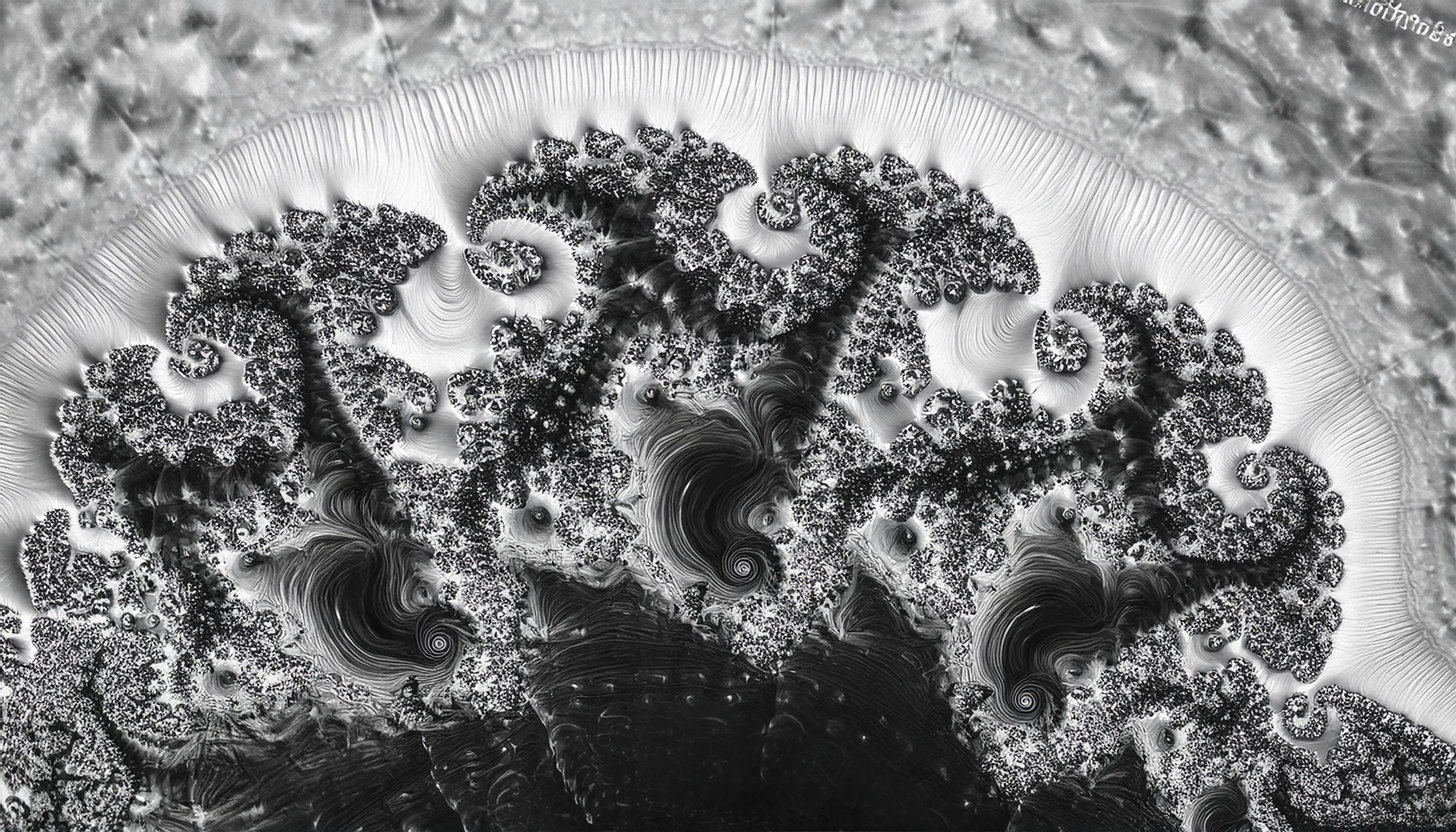
The Mandelbrot Set: Visualizing Infinity in Complexity
The Mandelbrot Set is generated by iterating the equation z = z² + c for each point on the complex plane. If the value of z escapes beyond a certain threshold within a set number of iterations, we color that point based on how quickly it diverges. If it stays bounded, we consider it part of the Mandelbrot Set and color it black.
Step 1: Basic Mandelbrot Set Visualization
To begin, we’ll set up a simple visualization that colors each point based on whether it is part of the Mandelbrot Set. We’ll iterate over each pixel in the canvas, treating each pixel as a point on the complex plane.
let maxIterations = 100;

function setup() {
  createCanvas(400, 400);
  pixelDensity(1);
  noLoop();
}

function draw() {
  loadPixels();
  for (let x = 0; x < width; x++) {
    for (let y = 0; y < height; y++) {

      // Map pixel position to a point in the complex plane
      let a = map(x, 0, width, -2.5, 1);
      let b = map(y, 0, height, -1, 1);
      let ca = a;
      let cb = b;

      let n = 0;
      let z = 0;
      while (n < maxIterations) {
        let aa = a * a - b * b;
        let bb = 2 * a * b;
        a = aa + ca;
        b = bb + cb;

        if (abs(a + b) > 16) {
          break; // Point has escaped
        }
        n++;
      }

      // Color based on the number of iterations
      let bright = map(n, 0, maxIterations, 0, 255);
      if (n === maxIterations) {
        bright = 0; // Point is in the Mandelbrot Set
      }

      let pix = (x + y * width) * 4;
      pixels[pix + 0] = bright;
      pixels[pix + 1] = bright;
      pixels[pix + 2] = bright;
      pixels[pix + 3] = 255;
    }
  }
  updatePixels();
}
Explanation of the Code
1. Mapping Coordinates: Each pixel’s coordinates (x, y) are mapped to a corresponding point (a, b) on the complex plane. This allows us to represent complex numbers on the canvas.
2. Iterations and Escaping: We iterate the equation z = z² + c up to maxIterations times. If the value escapes (its magnitude exceeds a certain threshold), we break the loop and record how quickly it diverged.
3. Coloring: Points that remain bounded are colored black, while diverging points are given a brightness level based on the number of iterations before they escaped. This creates the fractal-like edge where detail emerges.
Visual Transformation: A Basic Mandelbrot Fractal
This initial visualization gives us a basic Mandelbrot fractal. You’ll see the familiar black “body” of the Mandelbrot Set, surrounded by grayscale gradients representing points that escape at different rates. Even at this level, the fractal complexity is evident.
Step 2: Adding Color Gradients for Depth and Detail
To make the fractal more visually appealing, let’s add a color gradient to the diverging points. This will give the fractal more depth and help highlight the intricate boundary details.
function draw() {
  loadPixels();
  for (let x = 0; x < width; x++) {
    for (let y = 0; y < height; y++) {
      let a = map(x, 0, width, -2.5, 1);
      let b = map(y, 0, height, -1, 1);
      let ca = a;
      let cb = b;

      let n = 0;
      while (n < maxIterations) {
        let aa = a * a - b * b;
        let bb = 2 * a * b;
        a = aa + ca;
        b = bb + cb;

        if (abs(a + b) > 16) {
          break;
        }
        n++;
      }

      // Use HSB color mode for a gradient effect
      let hue = map(n, 0, maxIterations, 0, 255);
      let sat = 255;
      let bright = n === maxIterations ? 0 : 255;

      colorMode(HSB);
      let col = color(hue, sat, bright);
      let pix = (x + y * width) * 4;
      pixels[pix + 0] = red(col);
      pixels[pix + 1] = green(col);
      pixels[pix + 2] = blue(col);
      pixels[pix + 3] = 255;
    }
  }
  updatePixels();
}
Explanation of the Gradient Enhancement
1. HSB Color Mode: We use the HSB (Hue, Saturation, Brightness) color mode to create a gradient based on the number of iterations before escape. This adds color depth, making the fractal boundary more vibrant and visually complex.
2. Brightness for Bounded Points: Points within the Mandelbrot Set remain black, while points that escape are given a hue based on how quickly they diverge.
Visual Transformation: A Colorful Fractal Landscape
The Mandelbrot Set now displays vivid colors that make the boundaries pop. The gradient adds depth and highlights the intricate details of the fractal edges, revealing layers of complexity.
Step 3: Adding Zoom and Pan Functionality
To explore the Mandelbrot Set more closely, let’s add interactive zoom and pan functionality. This allows us to navigate deeper into the fractal, revealing self-similar patterns at different scales.
let zoom = 1;
let offsetX = 0;
let offsetY = 0;

function mouseWheel(event) {
  zoom *= event.delta > 0 ? 1.1 : 0.9;
  redraw();
}

function mouseDragged() {
  offsetX += movedX * 0.005 * zoom;
  offsetY += movedY * 0.005 * zoom;
  redraw();
}

function draw() {
  loadPixels();
  for (let x = 0; x < width; x++) {
    for (let y = 0; y < height; y++) {
      let a = map(x, 0, width, -2.5, 1) * zoom + offsetX;
      let b = map(y, 0, height, -1, 1) * zoom + offsetY;
      let ca = a;
      let cb = b;

      let n = 0;
      while (n < maxIterations) {
        let aa = a * a - b * b;
        let bb = 2 * a * b;
        a = aa + ca;
        b = bb + cb;

        if (abs(a + b) > 16) {
          break;
        }
        n++;
      }

      let hue = map(n, 0, maxIterations, 0, 255);
      let sat = 255;
      let bright = n === maxIterations ? 0 : 255;

      colorMode(HSB);
      let col = color(hue, sat, bright);
      let pix = (x + y * width) * 4;
      pixels[pix + 0] = red(col);
      pixels[pix + 1] = green(col);
      pixels[pix + 2] = blue(col);
      pixels[pix + 3] = 255;
    }
  }
  updatePixels();
}
Explanation of the Zoom and Pan Functions
1. Zooming with Mouse Wheel: The mouseWheel function adjusts the zoom variable, allowing us to zoom in and out of the fractal.
2. Panning with Mouse Drag: The mouseDragged function shifts offsetX and offsetY based on mouse movement, enabling us to move around the fractal at different zoom levels.
3. Redrawing with Zoom and Offset: In draw(), we apply zoom and offsets to a and b, effectively zooming in on the fractal and shifting the view.

Result: A Fully Interactive Mandelbrot Explorer
The final result is an interactive Mandelbrot Set visualization that allows for zooming and panning. As you zoom in, new details emerge, revealing self-similar patterns and endless complexity—a testament to the infinite nature of fractals.

Bringing It All Together: Creating Complex Art from Mathematical Elements
As we reach the end of this exploration into mathematical art, it’s time to bring together the various techniques we’ve discussed. Each method—whether it’s cellular automata, fractals, attractors, or noise functions—carries its own unique qualities, but combining them allows us to create artwork that’s greater than the sum of its parts. This section will serve as both a showcase and a guide on how to layer these mathematical elements into one complex, cohesive piece.
Showcase of Combined Techniques
Imagine a blank canvas as the beginning. We start with Perlin noise to add texture, giving the background a sense of organic variation—like mist rolling over a landscape or waves rippling across a body of water. The soft randomness of Perlin noise brings depth to the piece, establishing a base that mimics natural terrain or cloudy skies.

Next, we add structure with cellular automata. For instance, using cellular automata rules, we could define areas of contrast that resemble city grids or patterns in plant tissue, bringing an element of spatial structure to our textured background.
Then, we layer in Voronoi diagrams to partition space, creating regions that resemble natural cell structures or territories. The Voronoi cells add a fragmented look, dividing the art into unique segments, each contributing to the complexity of the overall composition.
As a finishing touch, we add chaotic attractors like the Lorenz Attractor, tracing looping paths across the canvas. These paths bring movement and a sense of unpredictability, looping and swirling through the structured spaces, adding an organic, flowing element that contrasts with the rigid structures created by Voronoi cells.
The result is a layered, intricate artwork—a world of organized chaos. From afar, it might resemble a landscape, a cellular network, or an abstract piece; yet, up close, the mathematical elements reveal themselves, each contributing to the harmony of the whole.
Reflection
In creating this piece, we see how different mathematical theories can combine to produce complexity that feels both intentional and organic. It’s a reminder that what appears chaotic or random often has underlying rules—an order hidden beneath the surface. The techniques we’ve explored don’t just represent individual functions or algorithms; they mirror natural processes, from the growth of plants to the unpredictable flow of fluids, showing that the world’s complexity is often rooted in simplicity.
This exploration of generative art reminds us that mathematics is more than equations; it’s a language for creating beauty, a way of capturing the structures and rhythms of the universe itself.
Conclusion: The Beauty of Order and Chaos in Art and Nature
As we conclude this journey through mathematical art, it’s clear that the harmony between order and chaos is a fundamental part of both nature and creativity. From the quiet complexity of fractals to the dynamic flow of attractors, we see that the same mathematical principles that describe our universe can also serve as tools for art.
Mathematics has often been associated with precision and rigidity, but here we see it as a medium of boundless creativity. Chaos and order, often seen as opposites, coexist beautifully in generative art, revealing the balance that underlies both life and the cosmos.
Invitation to Experiment
The tools and concepts we’ve explored are just the beginning. Generative art is accessible to anyone willing to experiment. With p5.js, a few lines of code can transform mathematical ideas into intricate, captivating images. Whether you’re a seasoned programmer or just starting, creating art from mathematics is both rewarding and enlightening. Each step, each iteration, brings new possibilities, allowing you to explore and experiment endlessly.
So go ahead—take these techniques, play with them, and make them your own. Whether you create patterns, landscapes, or entirely new forms, remember that you’re participating in something profound: the art of discovering the universe’s hidden structures, one line of code at a time.


Leave a comment